![<?echo $_SERVER['SERVER_NAME'];?>](/template/twentyseventeen/skin/images/header.jpg)
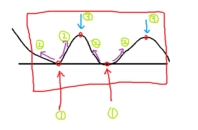
â€â€â€The image is represented by one-dimensional coordinates, 2D and 3D are not easy to draw, you must use matlab, I will not use it, the meaning can be expressed in place.
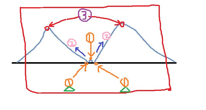
The first step: find the local minimum point of the image, this method is a lot, you can use a kernel to find, you can also compare one by one, it is not difficult to achieve.
Step 2: Start the water injection from the lowest point, the water begins to fill the net (the image is the gradient method), where the lowest points have been marked, will not be submerged, and those intermediate points are submerged.
The third step: find the local highest point, which is the two points corresponding to the 3 positions in the figure.
Step 4: This allows the image to be segmented based on the local minimum and the local maximum found.
Classification map
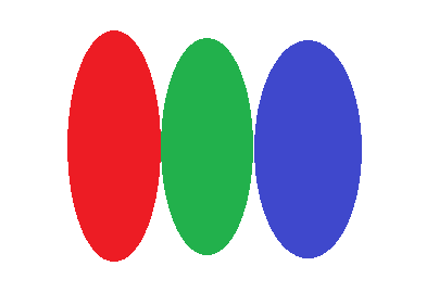
Simulation result graph
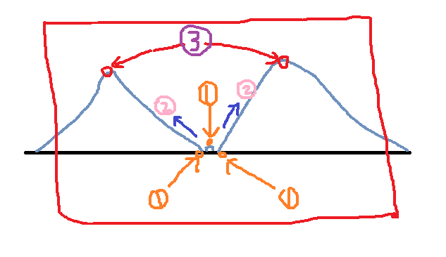
Does it feel that the above method is very good and simple? Then look at the picture below:
Using the above steps, the first step found three points, then the second step began to flood the water, all three points were recorded, and two local maxima were found.
Is this what we want?
The answer is no! We don't need the minimum value in the middle, because it's just a small and very small noise. We don't need to be as detailed as image segmentation.
The flaws are revealed? It doesn't matter, our opencv below solves this problem.
Analog classification map
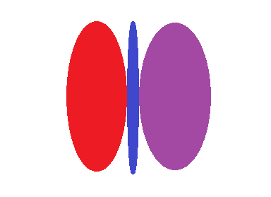
Simulation result graph
Opencv improved watershed algorithm:
In response to the above problems, we are thinking about whether we can mark this small detail so that it does not belong to the smallest point we find.
The improvement of opencv is the use of manual markup. We mark some points and use these points to guide the watershed algorithm. The effect is very good!
For example, we mark two triangles on the image above. In the first step, we find three local minimum points. When the second step is overwhelmed, all three points are overwhelmed. However, if the middle one is not marked, it will drown ( There are no lifebuoys, and the remaining two points are retained so that we can achieve the results we want.
Note: The markup here is made with different labels. I used the same triangle for convenience. Because tags are used for classification, different tags are labeled differently! This is reflected in the opencv program below. . .
Analog classification map
Simulation result graph
Note: The specific implementation is not completed. I feel that the principle will be used. I will study the algorithm when you need to go deep. When you understand the principle, you should change it. The interview is over. It’s ok! Hahaha~~
Opencv implementation:
#include
#include
Using namespace cv;
Using namespace std;
Void waterSegment(InputArray& _src, OutputArray& _dst, int& noOfSegment);
Int main(int argc, char** argv) {
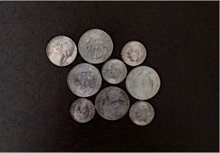
Mat inputImage = imread("coins.jpg");
Assert(!inputImage.data);
Mat graImage, outputImage;
Int offSegment;
waterSegment(inputImage, outputImage, offSegment);
waitKey(0);
Return 0;
}
Void waterSegment(InputArray& _src,OutputArray& _dst,int& noOfSegment)
{
Mat src = _src.getMat();//dst = _dst.getMat();
Mat grayImage;
cvtColor(src, grayImage, CV_BGR2GRAY);
Threshold(grayImage, grayImage, 0, 255, THRESH_BINARY | THRESH_OTSU);
Mat kernel = getStructuringElement(MORPH_RECT, Size(9, 9), Point(-1, -1));
morphologyEx(grayImage, grayImage, MORPH_CLOSE, kernel);
distanceTransform(grayImage, grayImage, DIST_L2, DIST_MASK_3, 5);
Normalize(grayImage, grayImage,0,1, NORM_MINMAX);
grayImage.convertTo(grayImage, CV_8UC1);
Threshold(grayImage, grayImage,0,255, THRESH_BINARY | THRESH_OTSU);
morphologyEx(grayImage, grayImage, MORPH_CLOSE, kernel);
Vector
Vector
Mat showImage = Mat::zeros(grayImage.size(), CV_32SC1);
findContours(grayImage, contours, hierarchy, RETR_TREE, CHAIN_APPROX_SIMPLE, Point(-1, -1));
For (size_t i = 0; i < contours.size(); i++)
{
//here static_cast
drawContours(showImage, contours, static_cast
}
Mat k = getStructuringElement(MORPH_RECT, Size(3, 3), Point(-1, -1));
morphologyEx(src, src, MORPH_ERODE, k);
Watershed(src, showImage);
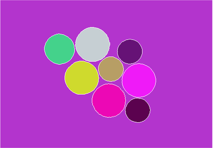
/ / Randomly assign color
Vector
For (size_t i = 0; i < contours.size(); i++) {
Int r = theRNG().uniform(0, 255);
Int g = theRNG().uniform(0, 255);
Int b = theRNG().uniform(0, 255);
Colors.push_back(Vec3b((uchar)b, (uchar)g, (uchar)r));
}
// show
Mat dst = Mat::zeros(showImage.size(), CV_8UC3);
Int index = 0;
For (int row = 0; row < showImage.rows; row++) {
For (int col = 0; col < showImage.cols; col++) {
Index = showImage.at
If (index > 0 && index <= contours.size()) {
Dst.at
}
Else if (index == -1)
{
Dst.at
}
Else {
Dst.at
}
}
}
}
Watershed merge code:
Void segMerge(Mat& image, Mat& segments, int& numSeg)
{
Vector
Int newNumSeg = numSeg;
/ / Initialize the length of the variable Vector
For (size_t i = 0; i < newNumSeg; i++)
{
Mat sample;
Samples.push_back(sample);
}
For (size_t i = 0; i < segments.rows; i++)
{
For (size_t j = 0; j < segments.cols; j++)
{
Int index = segments.at
If (index >= 0 && index <= newNumSeg)// merges points from the same area into one Mat
{
If (!samples[index].data)//The data is empty and cannot be merged, otherwise an error is reported.
{
Samples[index] = image(Rect(j, i, 1, 1));
}
Else / / merge by line
{
Vconcat(samples[index], image(Rect(j, i, 2, 1)), samples[index]);
}
}
//if (index >= 0 && index <= newNumSeg)
// samples[index].push_back(image(Rect(j, i, 1, 1)));
}
}
Vector
Mat hsv_base;
Int h_bins = 35;
Int s_bins = 30;
Int histSize[2] = { h_bins , s_bins };
Float h_range[2] = { 0,256 };
Float s_range[2] = { 0,180 };
Const float* range[2] = { h_range,s_range };
Int channels[2] = { 0,1 };
Mat hist_base;
For (size_t i = 1; i < numSeg; i++)
{
If (samples[i].dims > 0)
{
cvtColor(samples[i], hsv_base, CV_BGR2HSV);
calcHist(&hsv_base, 1, channels, Mat(), hist_base, 2, histSize, range);
Normalize(hist_base, hist_base, 0, 1, NORM_MINMAX);
Hist_bases.push_back(hist_base);
}
Else
{
Hist_bases.push_back(Mat());
}
}
Double similarity = 0;
Vector
For (size_t i = 0; i < hist_bases.size(); i++)
{
For (size_t j = i+1; j < hist_bases.size(); j++)
{
If (!merged[j])// unmerged areas for similarity judgment
{
If (hist_bases[i].dims > 0 && hist_bases[j].dims > 0)//This dimension is not necessary, just use a data.
{
Similarity = compareHist(hist_bases[i], hist_bases[j], HISTCMP_BHATTACHARYYA);
If (similarity > 0.8)
{
Merged[j] = true; / / merged area flag is true
If (i != j)// is not necessary here, i cannot be equal to j
{
newNumSeg --; / / split part reduction
For (size_t p = 0; p < segments.rows; p++)
{
For (size_t k = 0; k < segments.cols; k++)
{
Int index = segments.at
If (index == j) segments.at
}
}
}
}
}
}
}
}
numSeg = newNumSeg; / / return the number of regions after the merge
}
1. More than 12000 styles of data, which cover all models of front films, back films and full coverage back films. They are suitable for mobile phones, tablets, watches, cameras, and airpods, etc.
2. Can cut 12.9 inches of large films, and use it as you like.
3. Automatic film feeding with movie exit function, more convenient to operate.
4. Cloud data update, update models automatically.
5. Hole Position Precise. The screen protector film, which has been cut is perfect fitting with the phone screen.
6. Suitable for different types of TPH / TPU / 9H / INK film
7. Support phone x and y mirror
8. Support the cut explosion-proof film in the size of 0.35-0.37mm.
9. Support car rear view mirror film
10. Support blank Back Film DIY function
Screen Protection TPU Film Cutting Machine,Hydrogel Screen Protection Cutting Machine,high quality Mobile Phone Screen Protection,Mobile Phone Screen Protection Hydrogel Film Cutting Machine,Hydrogel Film Cutting Machine
Mietubl Global Supply Chain (Guangzhou) Co., Ltd. , https://www.mietublmachine.com