Detailed explanation of the neural network model processed by Python and Tensorflow

Recently, I tried to implement all the models of machine learning and deep learning in Python. The general learning ideas are as follows:

Classifier

Regression and prediction

sequentially

All models are first implemented in Python and then implemented in Tensorflow.

1 data set

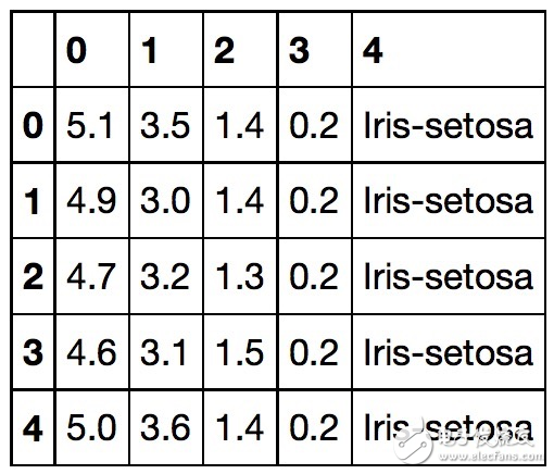
This paper begins with the Iris data set in UCI as the training data set and test time set. The data set gives the length and width of the sepel and the length and width of the petal. Based on these four characteristics, the model is predicted to predict the flower type (Iris Setosa, Iris Versicolour, Iris Virginica).
#包引
Import pandas as pd
Import numpy as np
Import matplotlib.pyplot as plt
Import os
Df = pd.read_csv('https://archive.ics.uci.edu/ml/machine-learning-databases/iris/iris.data', header=None)
Df.head(10)

1.1 Data Processing

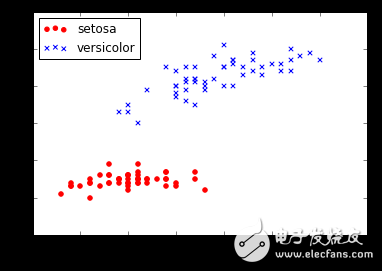
We extracted the first 100 samples (50 Iris Setosa and 50 Iris Versicolour) and labeled the different sample categories as 1 (Iris Versicolour) and -1 (Iris Setosa); then, the length of the flower buds and the length of the petals were taken as feature. The general treatment is as follows:
y = df.iloc[0:100, 4].values ​​# Forecast Label Vector
y = np.where(y == 'Iris-setosa', -1, 1)
X = df.iloc[0:100, [0,2]].values ​​# Input eigenvectors

# Visualization of samples using scatter plots
Plt.scatter(X[:50, 0], X[:50,1], color='red', marker='o', label='setosa')
Plt.scatter(X[50:100, 0], X[50:100, 1], color='blue', marker='x', label='versicolor')
Plt.xlabel('petal length')
Plt.ylabel('sepal length')
Plt.legend(loc='upper left')
Plt.show

2 model

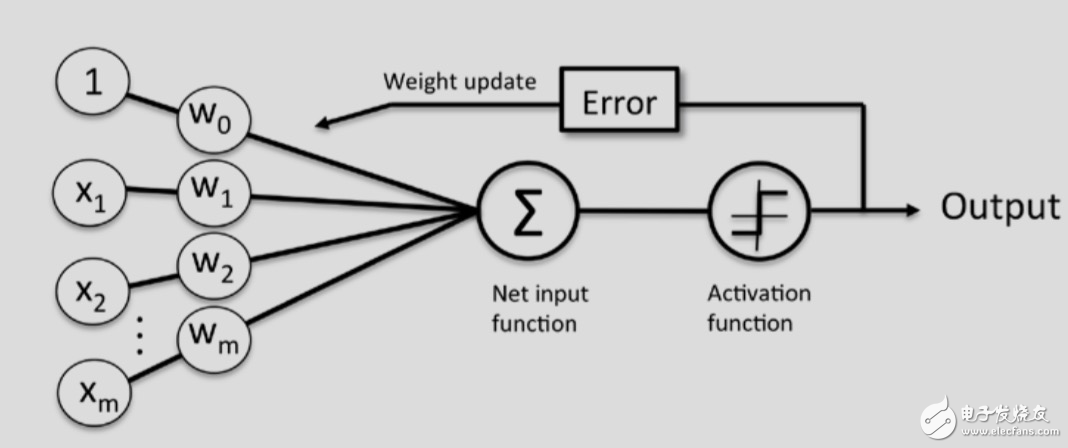
2.1 Neural network model

2.1.1 Model implementation

We can turn this problem into a two-category task, so 1 and -1 can be used as category labels. Thus the activation function can be expressed as follows:

The approximate model structure is as follows:

Class Perceptron(object):
"""
Parameters
------------
Eta : float
Learning rate (between 0.0 and 1.0)
N_iter : int
Number of iterations
Attributes
-----------
W_ : 1d-array
Weights
Errors_ : list
error
"""
Def __init__(self, eta=0.01, n_iter=10):
Self.eta = eta
Self.n_iter = n_iter

Def fit(self, X, y):
Self.w_ = np.zeros(1 + X.shape[1])
Self.errors_ = []

For _ in range(self.n_iter):
Errors = 0
For xi, target in zip(X, y):
Update = self.eta * (target - self.predict(xi))
Self.w_[1:] += update * xi
Self.w_[0] += update
Errors += int(update != 0.0)
Self.errors_.append(errors)
Return self

Def net_input(self, X):
Return np.dot(X, self.w_[1:]) + self.w_[0]

Def predict(self, X):
Return np.where(self.net_input(X) >= 0.0, 1, -1)

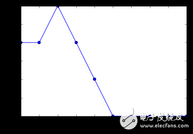
2.1.2 Model training
Ppn = Perceptron(eta=0.1, n_iter=10)
Ppn.fit(X, y)

2.1.3 Model verification

Error Analysis
Plt.plot(range(1, len(ppn.errors_) + 1), ppn.errors_, marker='o')
Plt.xlabel('Epochs')
Plt.ylabel('Number of misclassificaTIons')
Plt.show()

Visual classifier
From matplotlib.colors import ListedColormap
Def plot_decision_regions(X, y, classifier, resoluTIon=0.01):
"""
Visual classifier
:param X: sample feature vector
:param y: sample label vector
:param classifier: classifier
:param resoluTIon: residual
:return:
"""

Markers = ('s', 'x', 'o', '^', 'v')
Colors = ('red', 'blue', 'lightgreen', 'gray', 'cyan')
Cmap = ListedColormap(colors[:len(np.unique(y))])

X1_min, x1_max = X[:, 0].min() - 1, X[:, 0].max() + 1
X2_min, x2_max = X[:, 1].min() - 1, X[:, 1].max() + 1
Xx1, xx2 = np.meshgrid(np.arange(x1_min, x1_max, resoluTIon), np.arange(x2_min, x2_max, resolution))

Z = classifier.predict(np.array([xx1.ravel(), xx2.ravel()]).T)
Z = Z.reshape(xx2.min(), xx2.max())

Plt.contourf(xx1, xx2, Z, alpha=0.4, cmap=cmap)
Plt.xlim(xx1.min(), xx1.max())
Plt.ylim(xx2.min(), xx2.max())

For idx, cl in enumerate(np.unique(y)):
Plt.scatter(x=X[y == cl, 0], y=X[y == cl, 1], alpha=0.8, c=cmap(idx), marker=markers[idx], label=cl)

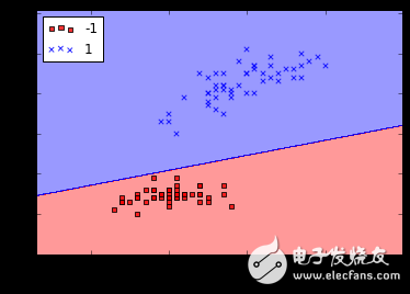
# Call visual classifier function
Plot_decision_regions(X, y, classifier=ppn)
Plt.xlabel('sepal length [cm]')
Plt.ylabel('petal length [cm]')
Plt.legend(loc='upper left')
Plt.show()

Fixed Series Outdoor Display

Products of Fixed Series Outdoor Display, the completive LED Display widely used in Outdoor Advertising Projects, like Square, Station, Commercial Center, Street etc. We Jongsun LED is specialized manufacturer from Shenzhen China, which focusing on the research and development, production, sales and engineering services of terminal LED Displays. We have the perfectly after-sales and 7x24hours technical support. Looking forward your cooperation!

Outdoor Led Display,Fixed Series Outdoor Display,Outdoor Full Color Led Display,Full Color Led Display

Shenzhen Jongsun Electronic Technology Co., Ltd. , https://www.jongsunled.com